Introduction

This is a project I started working on for my Machine Learning class. The aim, as you can read from the title, is being able to generate music that is, at least, not unpleasant.

In order to do so I investigated the use of Wasserstein Autoencoders (WAE), a generative model firstly proposed by Tolstikhin et al. ¹, which employs a regularizer derived from the theory of optimal transport.

The data

The data I used was published by a group of researchers from the Academia Sinica (Taiwan), as part of a paper² where they jointly proposed a novel GAN (MuseGAN) and released the dataset where the model was trained on. They open-sourced almost everything so you can access to their code and data.

This dataset contains 174154 unique 4/4 multi-track music pieces of 4 bars, coming from different rock music compositions. Every element of this dataset is represented as a multi-track (binary-valued) pianoroll. For those of you who are not familiar with DAWs or audio processing, a single-track pianoroll is basically a matrix whose entries represent the behaviour of the notes played by the single instrument. The number of columns in this matrix is the number of time-steps used to quantize the composition while the number of rows represents the octave extension, i.e. the number of possible notes that the instrument can execute.

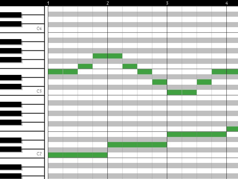
In this dataset a single bar is quantized into 48 time-steps (the minimum duration of a note is then 1/48th) and can span between 84 notes from C1 to B7. Every element of the dataset contains 4 bars of 5 instruments, resulting in a binary-valued (note on/off - velocity information is discarded) tensor of shape (4*48, 84, 5) = (192, 84, 5). The tempo was set to 100 bpm and the authors transposed every element to the same tonality. The instruments involved are Drums, Bass, Guitar, Piano and Strings.

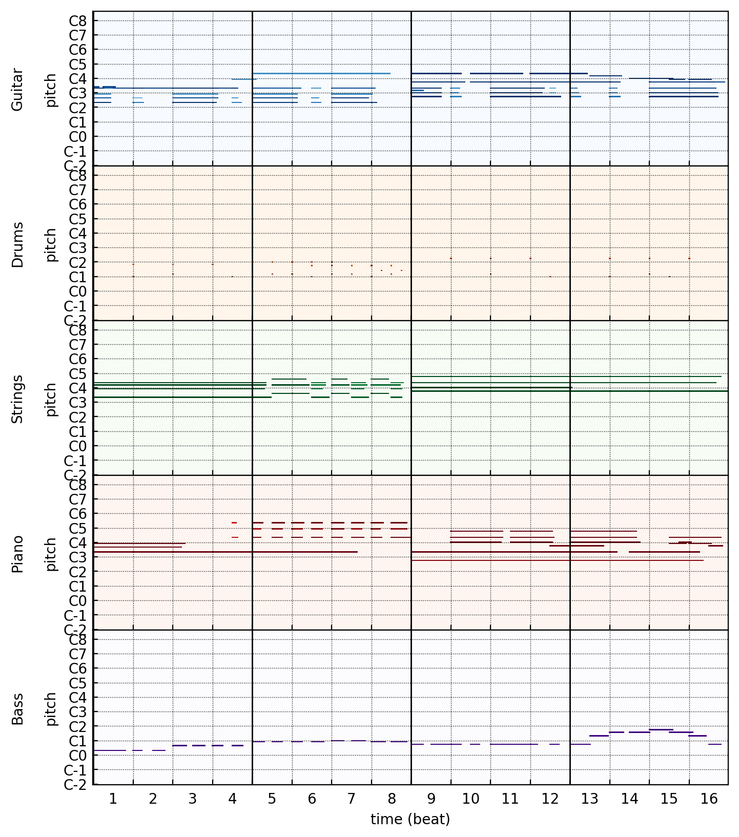
The pianoroll is one of the most commonly used representations, although it has some limitations. An important one, compared to the MIDI representation, is that there is no note-off information. As a result, there is no way to distinguish between a long note and repeated short notes. In order to partially solve this issue the authors did as following

Note that during the conversion from MIDI files to pianorolls, an additional minimal-length (of one time step) pause is added between two consecutive (without a pause) notes of the same pitch to distinguish them from one single note.

A few samples from the dataset³ (lower your audio output):

Theory

Disclaimer: a lot of this theory is taken from the original paper¹, I did not re-write it from scratch!

WAEs are a class of Autoencoders derived by theory of optimal transport. Given a collection of (unlabelled) data points $S_X$, the ultimate goal of the task is to tune a model capable of generating sets of synthetic points $S_G$ which look similar to $S_X$. There are various ways of defining the notion of similarity between two sets of data points: the most common approach assumes that both $S_X$ and $S_G$ are sampled independently from two probability distributions $P_X$ and $P_G$ respectively, and employ some of the known divergence measures for distributions.

Two major approaches currently dominate this field. Variational Auto-Encoders (VAEs) minimize the Kullback-Leibler (KL) divergence $D_{KL}(P_X, P_G)$, which is equivalent to maximizing the marginal log-likelihood of the model $P_G$. Generative Adversarial Networks (GANs) employ an elegant framework, commonly referred to as adversarial training, which is suitable for many different divergence measures, including (but not limited to) $f-$divergences, 1-Wasserstein distance, and Maximum Mean Discrepancy (MMD).

Similarly to VAEs, WAEs describe a particular way to train probabilistic latent variable models (LVMs) $P_G$. LVMs act by first sampling a code (feature) vector $Z$ from a prior distribution $P_Z$ defined over the latent space $\mathcal{Z}$ and then mapping it to a random input point $X \in \mathcal{X}$ using a conditional distribution $P_G(X|Z)$ also known as the decoder. This results is a density of the form

$$ p_G(x) = \int_{\mathcal{Z}} p_G(x|z)p(z)dz $$

assuming all involved densities are properly defined.

Instead of minimizing the KL divergence between the LVM $P_G$ and the unknown data distribution $P_X$ as done by VAEs, WAEs aim at minimizing any optimal transport distance between them. Kantorovich’s formulation of the optimal transport problem (OT) is given by

$$ W_c(P_X, P_G) = \inf_{\Gamma \in \mathcal{P}(X \sim P_X, Y \sim P_G)} \mathbb{E}_{(X,Y) \sim \Gamma} [c(X,Y)] $$

where $c:\mathcal{X} \times \mathcal{Y} \to \mathbb{R}^+$ is any measurable cost function and $\mathcal{P}(X \sim P_X, Y \sim P_G)$ is the set of all joint distributions of $(X, Y)$ with marginals $P_X$ and $P_G$ respectively. When $(\mathcal{X}, d)$ is a metric space (with distance $d$) and $c(x,y) = d^p(x,y)$ for $p \geq 1$ then $W_p$ (the $p$-th root of $W_c$) is known as the $p$-Wasserstein distance. When $p=1$ we then have the $1$-Wasserstein distance and this duality holds (Kantorovich-Rubinstein duality)

$$ W_1(P_X, P_G) = \sup_{f \in \mathcal{F}_L} \mathbb{E}_{X \sim P_X} [f(X)] - \mathbb{E}_{Y \sim P_G}[f(Y)] $$

where $\mathcal{F}_L$ is the set of all bounded 1-Lipschitz functions on $(\mathcal{X}, d)$. The authors state (and prove) that for deterministic decoders, i.e. $P_G(X|Z=z) = \delta_{G(z)}$ deterministically mapping latent codes $z \in \mathcal{Z}$ to the input space for a given map $G: \mathcal{Z} \to \mathcal{X}$, there is a simpler formulation for the OT problem: instead of finding a coupling $\Gamma$ between two random variables in $\mathcal{X}$ it is sufficient to find a conditional distribution $Q(Z|X)$ such that its $Z$ marginal $Q(Z) = \mathbb{E}_{X \sim P_X} [Q(Z|X)]$ is identical to the prior distribution $P_Z$. This resulted in a theorem where the OT problem was re-formulated (under these assumptions) as

$$ W_c(P_X, P_G) = \inf_{Q:Q_Z = P_Z} \mathbb{E}_{P_X}\big [ \mathbb{E}_{Q(Z|X)}[c(X, G(Z))] \big ] $$

In order to implement a numerical solution to this problem the authors relax the constraint on $Q_Z$ by adding a penalty term to the objective, which, in the end, takes the following form

$$ D_{WAE}(P_X, P_G) = \inf_{Q(Z|X) \in \mathcal{Q}} \mathbb{E}_{P_X}\big [ \mathbb{E}_{Q(Z|X)}[c(X, G(Z))] \big ] + \lambda \mathcal{D}_Z(Q_Z, P_Z) $$

where $\mathcal{Q}$ is any nonparametric set of probabilistic encoders, $\mathcal{D}_Z$ is an arbitrary divergence between $Q_Z$ and $P_Z$ , and $\lambda > 0$ is a hyperparameter. The authors propose two implementations of the WAE model, based on two different divergences.

WAE-GAN

The WAE-GAN model employs the Jensen-Shannon divergence, i.e.

$$ \mathcal{D}_Z(Q_Z, P_Z) = \mathcal{D}_{JS}(Q_Z, P_Z) = \frac{1}{2} D_{KL}(P_Z, M) + \frac{1}{2} D_{KL}(Q_Z, M) $$

where $M = \frac{1}{2}(P_Z + Q_Z)$ and uses the adversarial training to estimate it. The authors introduce an adversary (discriminator) in the latent space $\mathcal{Z}$ trying to separate “true” points sampled from $P_Z$ and “fake” ones sampled from $Q_Z$.

WAE-MMD

For a positive-definite reproducing kernel $k : \mathcal{X} \times \mathcal{X} \to \mathbb{R}$ the following expression is called the Maximum Mean Discrepancy (MMD):

$$ \text{MMD}_k(P_Z, Q_Z) = \Big | \Big | \int_\mathcal{Z} k(z, \cdot) dP_Z(z) - \int_\mathcal{Z} k(z, \cdot) dQ_Z(z) \Big | \Big |_{\mathcal{H}_k} $$

where $\mathcal{H}_k$ is the RKHS of real-valued functions mapping $\mathcal{Z}$ to $\mathcal{R}$. If $k$ is characteristic then MMD$_k$ defines a metric and can be used as a divergence measure. The authors propose to use an unbiased estimate of the MMD that is the sum of two $U$-statistics and a sample average. Given i.i.d. samples $\mathbf{P} = { z_1, \dots, z_n }$ from $P_Z$ and i.i.d. samples $\mathbf{Q} = {\tilde{z}_1, \dots, \tilde{z}_n}$ from $Q(Z|z_i)$ , the unbiased estimate⁴ is

$$ \widehat{MMD}^2_U \big [\mathcal{H}_k, \mathbf{P}, \mathbf{Q} \big ] = \frac{1}{n(n-1)} \sum_{i=1}^n \sum_{j \neq i} k(z_i, z_j) + \sum_{i=1}^n \sum_{j \neq i} k(\tilde{z}_i, \tilde{z}_j) - \frac{2}{n^2} \sum_{i=1}^n \sum_{j=1}^n k(z_i, \tilde{z}_j) $$

Experiments details

Architechtures

Encoder $Q_\phi$, decoder $G_{\theta}$ and discriminator $D_{\gamma}$ are parametrized by deep neural nets. Given the structure of the data, binary-valued tensors of shape (H,W,5) (where 5, the number of instruments, plays naturally the role of the number of channels), both encoder and decoder are CNNs, while the discriminator (which acts in the latent space $\mathcal{Z}$) is a “vanilla” NN. You can check out the various models I’ve coded here, they are almost all equals except for the strides of the convolutions.

The main architecture I used was inspired by DCGAN ⁵. In the following picture I’m showing the encoder that, starting from the (192, 84, 5) input tensor, applies 4 convolutions with $[6,6]$ filters, followed by Batch Normalizations and ReLUs. The last layer employs a reshape (not shown in the picture) followed by a (small dropout of 0.2 and a) fully-connected layer that maps the previous inputs into a vector of size $dim(\mathcal{Z}) = d_{\mathcal{Z}}$ (in the following picture $d_{\mathcal{Z}} = 8$).

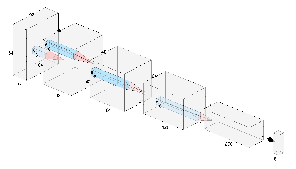
The decoder acts simmetrically wrt the encoder, using 2D transposed convolutions instead of convolutions. The discriminator network maps a vector from $\mathcal{Z}$ to $[0,1]$ through 6 dense layers followed by ReLUs.

Prior

I’ve used a Gaussian prior $P_Z = \mathcal{N} \big ( 0, \sigma_z^2 \cdot I_{d_z} \big )$ where the variance $\sigma_z^2$ is an hyperparameter.

Latent space dimensionality

The authors studied the choice of the dimensionality of the latent space in a follow-up paper⁶. They investigated the relationship between the latent space dimension $d_{\mathcal{Z}}$ and the *intrinsic dimensionality* of the data distribution, $d_{\mathcal{I}}$. This last quantity is, informally, *the minimum number of parameters required to continuously parametrise the data manifold*. If this quantity is greater than $d_{\mathcal{Z}}$ then the encoder will map the data distribution $P_X$ to $Q_Z$ supported on a latent manifold of dimension at most $d_{\mathcal{I}}$ while the divergence regularizer $\lambda \mathcal{D}_Z (Q_Z, P_Z)$ will encourage the encoder to fill the latent space similarly to the prior $P_Z$ as much as possible. This can potentially lead to the absence of any learning capability.

Adversarial training

I’ve decided to use (as the authors suggest) the non-saturating GAN loss ⁷: this resulted in a discriminator $D_\gamma$ trained by the maximization of

$$ \frac{\lambda}{n} \sum_{i=1}^n \log D_\gamma(z_i) + \log D_\gamma(1-\tilde{z}_i) $$

and in an autoencoder ($Q_\phi, G_\theta$) trained by the minimization of

$$ \frac{1}{n}\sum_{i=1}^n c(z_i, G_\theta(\tilde{z}_i)) - \lambda D_\gamma \log (\tilde{z}_i) $$

As the authors point out this procedure falls into the min-max problem which makes GAN unstable. This training strategy can then possibly yield instabilities in the training phase but the authors claim that by executing an adversarial training in a “simpler” space (wrt the pixel space where GANs are usually trained on), the whole process could benefit.

Cost function

I’ve used $c(x, y) = || x - y ||_2^2$ for both implementations (WAE-GAN and WAE-MMD).

Hyperparameters

Since there is no objective measure of performace for this kind of task, running an hyperparameter optimization procedure is hard. I’ve adjusted the parameters manually and so the results I obtained might not be the best that these model can produce.

Results

As mentioned in the data section, the input samples are binary-valued tensors of shape (192, 84, 5). The decoder, although, maps a latent code into $[0, 1]^{192 \times 84 \times 5}$ through the action of the sigmoid function. These output tensors $\hat{x}$ must then be binarized, and I’ve tried two strategies to do so:

1. Hard thresholding (HT): The resulting tensor entry $\hat{x}_{ijk}$ needs to be greater than a fixed threshold (0.5) in order to be mapped to 1. $$\hat{x}_{ijk}^{HT} = \begin{cases} 1 & \text{if } \hspace{10pt} x_{ijk} > 0.5 \\
   0 & \text {o.w }\end{cases}$$

2. Bernoulli sampling (BS) (by the authors of MuseGAN): The resulting tensor entry $\hat{x}_{ijk}$ needs to be greater than a sample from the uniform distribution over scalars between 0 and 1. $$\hat{x}_{ijk}^{BS} = \begin{cases} 1 & \text{if } \hspace{10pt} x_{ijk} > b \sim \mathcal{U}[0,1] \\
   0 & \text {o.w }\end{cases}$$

I’m presenting samples binarized with the HT method.

---

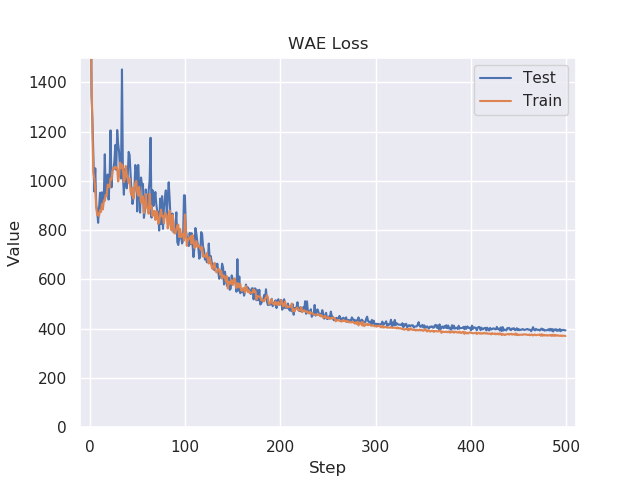
For a “fair” comparison the following results have been obtained with the same architecture and hyperparameters. Both WAE-GAN and WAE-MMD models have been trained with a latent dimension of $d_{\mathcal{Z}} = 128$. The number of filters in the four convolutions (see the picture above) are [8, 16, 32, 64] for the encoder and [64, 32, 16, 8] for the decoder. Both sequences of convolution used a fixed filter size of 6x6. I’ve trained both models for 500 epochs with Adam. Both autoencoder’s and discriminator’s optimizer started with a learning rate of $10^{-4}$ and both employed a decay to $\approx 10^{-5}$.

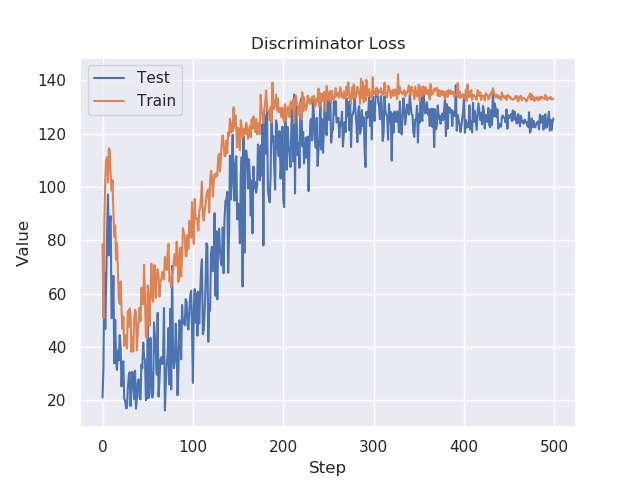
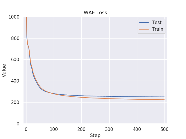
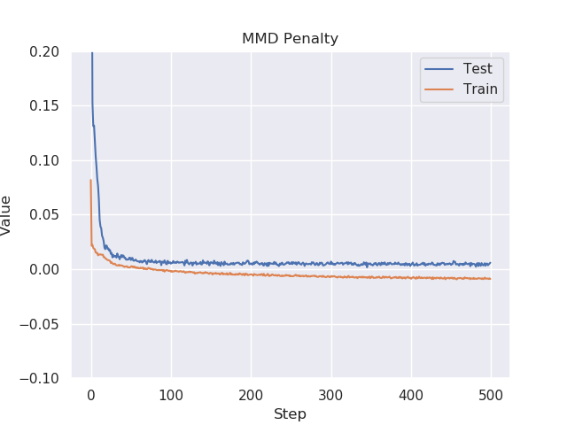
Random Generation

The following are a few of the “best” samples (wrt my personal taste) that I picked: please make sure to lower the level of your audio output³ before playing! I suggest listening with headphones.

WAE-GAN	WAE-MMD

The samples I was able to generete lightly suffer the problem of over-fragmentation. The notes generated tend to be fragmented, sometimes yielding chaotic and unpleasant results. This problem has also been recognized in ² and the authors of MuseGAN proposed a new version of the model where their generator was equipped with binary neurons⁸, making it able to map the input noise directly into binary-valued output tensors. This partially solved the issue.

In my opinion WAE-GAN was able to produce better results: this was also the opinion of the authors of WAE.

Reconstruction

These are a few reconstructed samples from the test set.

Original Sample	WAE-GAN	WAE-MMD

Qualitatively speaking both models gave comparable results in terms of recostruction capabilities. It’s clear that they both struggle reconstructing the drums. Drums events are more sparse and they might need wider (and possibly more) filters in order to be reconstructed clearly.

References

---

1. Wasserstein Auto-Encoders ↩︎

2. MuseGAN: Multi-track Sequential Generative Adversarial Networks for Symbolic Music Generation and Accompaniment ↩︎

3. I’ve done the MIDI to MP3 conversions with the help of VLC and its integrated synthesizer FluidSynth. I’ve done no post-processing (eq, fx, mixing, mastering) so what you hear comes straight out-of-the box. The sounds produced are unpleasant: please think of them as part of an experiment and not music meant to be played. ↩︎

4. Kernel Mean Embedding of Distributions: A Review and Beyond page 52 ↩︎

5. Unsupervised Representation Learning with Deep Convolutional Generative Adversarial Networks ↩︎

6. On the Latent Space of Wasserstein Auto-Encoders ↩︎

7. Are GANs Created Equal? A Large-Scale Study ↩︎

8. Convolutional Generative Adversarial Networks with Binary Neurons for Polyphonic Music Generation ↩︎